Closed-loop transfer function

To overcome the limitations of the open-loop controller, control theory introduces feedback. A closed-loop controller uses feedback to control states or outputs of a dynamical system. Its name comes from the information path in the system: process inputs (e.g., voltage applied to an electric motor) have an effect on the process outputs (e.g., speed or torque of the motor), which is measured with sensors and processed by the controller; the result (the control signal) is "fed back" as input to the process, closing the loop.

Closed-loop controllers have the following advantages over open-loop controllers:

• disturbance rejection (such as hills in the cruise control example above)

• guaranteed performance even with model uncertainties, when the model structure does not match perfectly the real process and the model parameters are not exact

• unstable processes can be stabilized

• reduced sensitivity to parameter variations

• improved reference tracking performance

In some systems, closed-loop and open-loop control are used simultaneously. In such systems, the open-loop control is termed feedforward and serves to further improve reference tracking performance.

A common closed-loop controller architecture is the PID controller.

Closed-loop transfer function

The output of the system y(t) is fed back through a sensor measurement F to a comparison with the reference value r(t). The controller C then takes the error e (difference) between the reference and the output to change the inputs u to the system under control P. This is shown in the figure. This kind of controller is a closed-loop controller or feedback controller.

This is called a single-input-single-output (SISO) control system; MIMO (i.e., Multi-Input-Multi-Output) systems, with more than one input/output, are common. In such cases variables are represented through vectors instead of simple scalar values. For some distributed parameter systems the vectors may be infinite-dimensional (typically functions).

If we assume the controller C, the plant P, and the sensor F are linear and time-invariant (i.e., elements of their transfer function C(s), P(s), and F(s) do not depend on time), the systems above can be analysed using the Laplace transform on the variables. This gives the following relations:

${\displaystyle Y(s)=P(s)U(s)\,\!}$

${\displaystyle U(s)=C(s)E(s)\,\!}$

${\displaystyle E(s)=R(s)-F(s)Y(s).\,\!}$

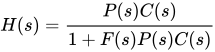
Solving for Y(s) in terms of R(s) gives

${\displaystyle Y(s)=\left({\frac {P(s)C(s)}{1+F(s)P(s)C(s)}}\right)R(s)=H(s)R(s).}$

The expression ${\displaystyle H(s)={\frac {P(s)C(s)}{1+F(s)P(s)C(s)}}}$ is referred to as the closed-loop transfer function of the system. The numerator is the forward (open-loop) gain from r to y, and the denominator is one plus the gain in going around the feedback loop, the so-called loop gain. If ${\displaystyle |P(s)C(s)|\gg 1}$, i.e., it has a large norm with each value of s, and if ${\displaystyle |F(s)|\approx 1}$, then Y(s) is approximately equal to R(s) and the output closely tracks the reference input.